Page 116 - DCOM303_DMGT504_OPERATION_RESEARCH

Unit 5: Transportation Problem

Notes
!
Caution The initial solution obtained by any of the three methods must satisfy the following
conditions.

1. The solution must be feasible, i.e., the supply and demand constraints must be
satisfied (also known as rim conditions).
2. The number of positive allocations, N must be equal to m + n – 1, where m is the
number of rows and n is the number of columns.

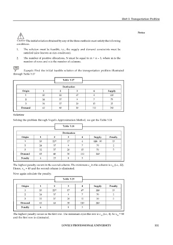
Example: Find the initial feasible solution of the transportation problem illustrated
through Table 5.17

Table 5.17

Destination
Origin 1 2 3 4 Supply
1 20 22 17 4 120
2 24 37 9 7 75
3 34 37 20 15 25
Demand 60 40 30 110 240

Solution:
Solving the problem through Vogel's Approximation Method, we get the Table 5.18

Table 5.18

Destination
Origin 1 2 3 4 Supply Penalty
40
1 20 22 17 4 120 80 13
2 24 37 9 7 70 2
3 32 37 20 15 50 5
Demand 60 40 30 110 240
Penalty 4 15 8 3

The highest penalty occurs in the second column. The minimum c in this column is c (i.e., 22).
ij 12
Hence, x = 40 and the second column is eliminated.
12
Now again calculate the penalty.
Table 5.19

Origin 1 2 3 4 Supply Penalty
1 20 22 17 4 120 13
80
40
2 24 37 9 7 70 2
3 32 37 20 15 50 5
Demand 60 40 30 110 240
Penalty 4 8 3

The highest penalty occurs in the first row. The minimum cij in this row is c (i.e., 4). So x = 80
14 14
and the first row is eliminated.
LOVELY PROFESSIONAL UNIVERSITY 111