Page 300 - DCOM303_DMGT504_OPERATION_RESEARCH

Unit 14: Decision-making

14.4.4 Equally likely Decision Criterion Notes

The equally likely decision criterion is based on the principle of insufficient reason and is
attributed to Laplace and thus, this criterion is also known as Laplace criteria. The approach
assumes that the decision maker has no knowledge as to which event will occur, and thus he
considers the likelihood of the different events occurring as being equal. In effect, the decision
maker has assigned the same probability value to each event. This probability is equal to
1/number of events. Hence, an average or expected payoff can be computed for each possible
strategy and the optimal decision will be the one with the best average payoff value.

Steps for Decision under Laplace Criteria

The formal procedure for finding the equally likely decision is as follows:
1. For each possible strategy, find the average or expected payoff by adding all the possible
payoffs and dividing by the number of possible events. Record this number in a new
column.
2. Select the strategy with the best average payoff value: maximum for profit and minimum
for cost.

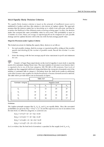
Example: A Super Bazar must decide on the level of supplies it must stock to meet the
needs of its customers during Diwali days. The exact number of customers is not known, but it
is expected to be in one of the four categories; 300, 350, 400 or 450 customers. Four levels of
supplies are thus suggested with level j being ideal (from the viewpoint of incurred costs) if the
number of customers falls in category j. Deviations from the ideal levels results in additional
costs either because extra supplies are stocked needlessly or because demand cannot be satisfied.
The table below provides these costs in thousands of rupees.
Table 14.3

Customer category Supplies level
A A A A
1 1 4
E 7 12 20 27
1
E 10 9 10 25
2
E 23 20 14 23
3
E 32 24 21 17
4

Solution:
The Laplace principle assumes that E , E , E , and E are equally likely. Thus, the associated
1 2 3 4
probabilities are given by P(E) = ¼¼ (j = 1, 2, 3, 4) and the expected costs due to deviations from
j
the best level, for different categories of customers are:
E(A ) = ¼ ¼¼(7 + 10 + 23 + 32) = 18.00
1
E(A ) = ¼ ¼¼(12 + 9 + 20 + 24) = 16.25
2
E(A ) = ¼ ¼¼(20 + 10 + 14 + 21) = 16.25
3
E(A ) = ¼ ¼¼(27 + 25 + 23 + 17) = 23.00
4
As it is evident, that the best level of inventory is specified by the supply level A or A .
2 3

LOVELY PROFESSIONAL UNIVERSITY 295