Page 142 - DLIS401_METHODOLOGY_OF_RESEARCH_AND_STATISTICAL_TECHNIQUES

Unit 9: Presentation of Data

9.3.4 Cumulative Frequency Curve or Ogive Notes

For plotting a cumulative frequency curve or Ogive, first of all cumulative frequencies against
each of the intervals are to be written. If we take the frequency distribution of Table 9.5, it will
be as shown in Table 9.6.
Table 9.6 Cumulative Frequency Distribution of Scores

Scores Frequency Cumulative Frequency
30–39 7 7
40–49 18 25

50–59 21 46
60–69 25 71
70–79 20 91
80–89 18 109
90–99 11 120

For getting the cumulative frequencies of a C.I. we take the cumulative frequencies upto the
previous interval and add the frequency of that interval into it. Here C.F. indicates that upto
39.5 there are 7 cases, upto 49.5 there are 25 cases, upto 59.5 there are 46 cases, and so on. The
difference between the construction of the frequency polygon and ogive is that for frequency
polygon, one takes the mid points of the C.I. on horizontal axis, while for ogive one takes the
upper boundary of the C.I. on horizontal axis. Again on the vertical axis, in case of Ogive one
takes cumulative frequency/cumulative percentage instead of frequency only. The cumulative
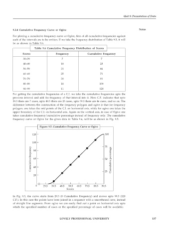
frequency curve or Ogive for the given data in Table 9.6, will be as shown in Fig. 9.5.

Figure: 9.5. Cumulative Frequency Curve or Ogive

120 100

100 75
frequency 80 percentage

Cumulative 60 50 Cumulative

40

20 25

0 29.5 39.5 49.5 59.5 69.5 79.5 89.5 99.5
Scores

In Fig. 9.5, the curve starts from 29.5 (0 Cumulative Frequency) and moves upto 99.5 (120
C.F.). In this case the points have been joined in a sequence with a smoothened cuve, instead
of straight line segments. From ogive we can easily find out a point on horizontal axis upto
which the specified number of cases or the specified percentage of cases will be available.

LOVELY PROFESSIONAL UNIVERSITY 137