Page 185 - DECO504_STATISTICAL_METHODS_IN_ECONOMICS_ENGLISH

Unit 12 : Linear Regression Analysis : Introduction and Lines of Regression

Notes
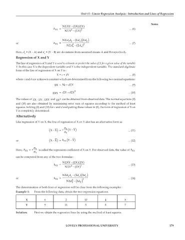
Σ NXY ( − )Σ ( X Y )Σ
b YX = 2 ... (6)
Σ NX 2 ( − X )Σ

N Σ − ( xy x )Σ dd ( d d y ) Σ
or b YX = 2 2 ... (7)
x − ( Σ N d d x )Σ

Here, d = (X – A) and d = (Y – B) are deviations from assumed means A and B respectively.
x y
Regression of X and Y
The line of regression of X and Y is used to estimate or predict the value of X for a given value of the variable
Y. In this case X is the dependent variable and Y is the independent variable. The standard algebraic
form of the line of regression of X on Y is :
X= c + dY ... (8)
where c and d are unknown constant which are determined from the following two normal equations:
+ΣY
ΣX = Ncd ... (9)
ΣXY = Σ+ ΣYc d Y 2 ... (10)

The values of ΣX , ΣY , ΣXY and ΣY 2 can be obtained from observed data. The normal equations (9)
and (10) are also obtained by minimising error sum of squares according to the method of least
squares. Solving (9) and (10) for c and d and putting these values in (8), the form of regression of X on
Y is completely determined.
Alternatively

Like regression of Y on X, the line of regression of X on Y also has an alternative form as
( − X = σ X Y ( r YY ) − ... (11)
) X
σ

) X
or ( − X = XY ( b YY ) − ... (12)
σ
Here, b XY = r X is called the regression coefficient of X on Y. For observed data, the value of b XY
σ Y
can be computed from any of the two formulae :
Σ Ν ( −XY )Σ ( Y )ΣX
b XY = Σ Ν 2 ( −Y Y )Σ 2 ... (13)

Ν Σ xy ( −dd x )Σ ( d d y ) Σ
or b XY = 2 2 ... (14)
y −d ( Σ Ν d y ) Σ

The determination of both lines of regression will be clear from the following examples :
Example 1: From the following data, obtain the two regression equations.

X 6 2 10 4 8
Y 9 11 5 8 7

Solution: First we obtain the regression lines by using the method of least squares.

LOVELY PROFESSIONAL UNIVERSITY 179