Page 187 - DECO504_STATISTICAL_METHODS_IN_ECONOMICS_ENGLISH

Unit 12 : Linear Regression Analysis : Introduction and Lines of Regression

– 26 = 20d ∴ d = – 1.3 Notes
Putting d = – 1.3 in equation (x),
30 = 5c + 40 × (– 1.3) or 5c = 30 + 52 = 82
∴ c = 16.4
Putting the values of c and d in (vii), the line of regression of X on Y is :
X = 16.4 – 1.3 Y
∴ X + 1.3 Y = 16.4
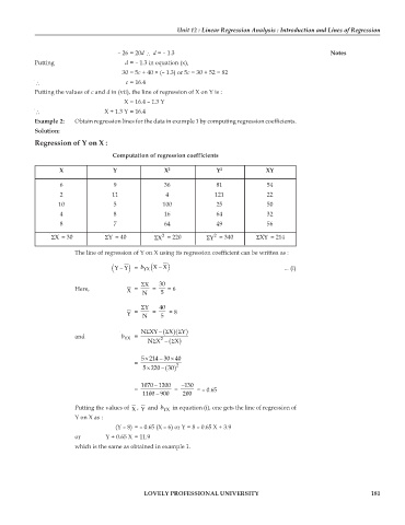
Example 2: Obtain regression lines for the data in example 1 by computing regression coefficients.
Solution:
Regression of Y on X :

Computation of regression coefficients
X Y X 2 Y 2 XY

6 9 36 81 54
2 11 4 121 22
10 5 100 25 50
4 8 16 64 32
8 7 64 49 56
2
2
ΣX = 30 ΣY = 40 ΣX = 220 ΣY = 340 ΣXY = 214
The line of regression of Y on X using its regression coefficient can be written as :
( YY ) − = YX ( b − X ) X ... (i)

ΣX 30
Here, X = N = 5 = 6

ΣY 40
Y = N = 5 = 8

Σ NXY ( − )Σ ( Y )ΣX
and b YX = Σ NX 2 ( − X )Σ

×
5 × − 214 30 40
= 2
5 × ( − 220 )30
1070 − 1200 −130
= = = – 0.65
1100 − 900 200
Putting the values of X Y and b YX in equation (i), one gets the line of regression of
,
Y on X as :
(Y – 8) = – 0.65 (X – 6) or Y = 8 – 0.65 X + 3.9
or Y + 0.65 X = 11.9
which is the same as obtained in example 1.

LOVELY PROFESSIONAL UNIVERSITY 181