Page 310 - DECO504_STATISTICAL_METHODS_IN_ECONOMICS_ENGLISH

Unit 24: Time Series Methods—Principle of Least Square and Its Application
Pavitar Parkash Singh, LPU

Unit 24: Time Series Methods—Principle of Least Notes

Square and Its Application

CONTENTS
Objectives
Introduction
24.1 Principle of Least Square and its Application
24.2 Merits, Demerits and Limitations of the Method of Least Square
24.3 Summary
24.4 Key-Words
24.5 Review Questions
24.6 Further Readings

Objectives

After reading this unit students will be able to:
• Explain the Principle of Least Square and its Applications.
• Know Merits, Demerits and Limitations of the Method of Least Square.
Introduction

The earlier discussed methods for trend analysis have certain defects, particularly in providing a
satisfactory projection for the future. To overcome this defect, a convenient method is to follow a
mathematical approach. The device for getting an objective fit of a straight line to a series of data is
the least squares method. It is perhaps the most commonly employed and a very satisfactory method
to describe the trend. The Mark off theorem states that for a given condition, the line fitted by the
method of least squares is the line of “best” fit in a well-defined sense. The term “best” is used to
mean that the estimates of the constants a and b are the best linear unbiased estimates of those constants.
24.1 Principle of Least Square and its Application

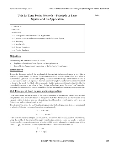
In the least squares method, the sum of the vertical deviations of the observed values from the fitted
straight line is zero. Secondly, the sum of the squares of all these deviations is less than the sum of the
squared vertical deviations from any other straight line. The method of least squares can be used for
fitting linear and non-linear trends as well.
To determine the values of a and b in a linear equation by the least squares method, we are required
to solve the following two normal equations simultaneously:
∑Y = an b ∑X
+
∑XY = a ∑ ∑X + b X 2
In the case of time series analysis, the solution of a and b from these two equations is simplified by
using the middle of the series as the origin. Since the time units in a series are usually of uniform
duration and are consecutive numbers, when the middle point is taken as the origin, the sum of time
units, i.e., ∑X , will be zero. As a result, the above two normal equations reduce to:
∑Y = an
∑XY = b∑ X 2

LOVELY PROFESSIONAL UNIVERSITY 305