Page 314 - DECO504_STATISTICAL_METHODS_IN_ECONOMICS_ENGLISH

Unit 24: Time Series Methods—Principle of Least Square and Its Application

If the middle of the time series is taken as origin, as done earlier, the above normal Notes
equations reduce to
+
∑Y = na c ∑X 2
∑XY = ∑Xb 2

2
∑XY = ∑ a 2 +X ∑ c X 4
Simplifying, we get:

2
n ∑ XY – X ∑ ∑ 2 Y
c = 2 ... (7)
n ∑ 4 ( X– ∑ 2 ) X

∑ ∑Y – c X 2
a = ... (8)
n
∑XY
b = ... (9)
∑X 2
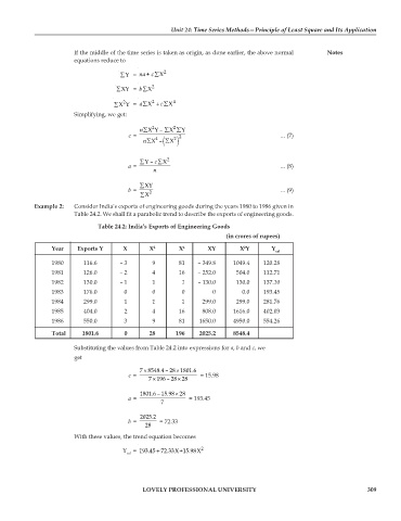
Example 2: Consider India’s exports of engineering goods during the years 1980 to 1986 given in
Table 24.2. We shall fit a parabolic trend to describe the exports of engineering goods.
Table 24.2: India’s Exports of Engineering Goods
(in crores of rupees)
Year Exports Y X X 2 X 4 XY X Y Y
2
cal
1980 116.6 – 3 9 81 – 349.8 1049.4 120.28
1981 126.0 – 2 4 16 – 252.0 504.0 112.71
1982 130.0 – 1 1 1 – 130.0 130.0 137.10
1983 176.0 0 0 0 0 0.0 193.45
1984 299.0 1 1 1 299.0 299.0 281.76
1985 404.0 2 4 16 808.0 1616.0 402.03
1986 550.0 3 9 81 1650.0 4950.0 554.26

Total 1801.6 0 28 196 2025.2 8548.4
Substituting the values from Table 24.2 into expressions for a, b and c, we
get

7 × × 8548.4 – 28 1801.6
c = = 15.98
×
×
7196 – 28 28
1801.6 – 15.98 × 28
a = = 193.45
7
2025.2
b = = 72.33
28
With these values, the trend equation becomes

2
Y = 193.45 72.33X+15.98X
+
cal

LOVELY PROFESSIONAL UNIVERSITY 309