Page 317 - DECO504_STATISTICAL_METHODS_IN_ECONOMICS_ENGLISH

Statistical Methods in Economics

Notes Solution:

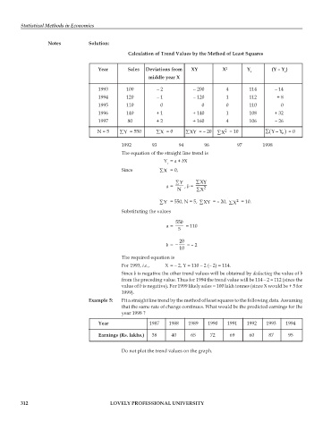
Calculation of Trend Values by the Method of Least Squares

Year Sales Deviations from XY X 2 Y (Y – Y )
c c
middle year X

1993 100 – 2 – 200 4 114 – 14
1994 120 – 1 – 120 1 112 + 8
1995 110 0 0 0 110 0
1996 140 + 1 + 140 1 108 + 32
1997 80 + 2 + 160 4 106 – 26
)
N = 5 ∑Y = 550 ∑X = 0 ∑XY = – 20 ∑X = 10 ∑ ( − YY = 0
2
c
1992 93 94 96 97 1998
The equation of the straight line trend is
Y = a + bX
c
Since ∑X = 0,

∑Y ∑XY
a = , b =
N ∑X 2

2
∑Y = 550, N = 5, ∑XY = – 20, ∑X = 10.
Substituting the values

550
a = = 110
5
20
b = − = – 2
10
The required equation is
For 1993, i.e., X = – 2, Y = 110 – 2 (– 2) = 114.
Since b is negative the other trend values will be obtained by deducting the value of b
from the preceding value. Thus for 1994 the trend value will be 114 – 2 = 112 (since the
value of b is negative). For 1999 likely sales = 100 lakh tonnes (since X would be + 5 for
1999).
Example 5: Fit a straight line trend by the method of least squares to the following data. Assuming
that the same rate of change continues. What would be the predicted earnings for the
year 1998 ?
Year 1987 1988 1989 1990 1991 1992 1993 1994

Earnings (Rs. lakhs.) 38 40 65 72 69 60 87 95

Do not plot the trend values on the graph.

312 LOVELY PROFESSIONAL UNIVERSITY