Page 316 - DECO504_STATISTICAL_METHODS_IN_ECONOMICS_ENGLISH

Unit 24: Time Series Methods—Principle of Least Square and Its Application

Notes
630
∴ a = = 90
7
56
and b = = 2
28
Hence the equation of the straight line trend is
Y = 90 + 2X
c
For X = – 3, Y = 90 + 2 (– 3) = 84
c
For X = – 2, Y = 90 + 2 (– 2) = 86
c
For X = – 1, Y = 90 + 2 (– 1) = 88
c
Similarly, by putting X = 0, 1, 2, 3, we can obtain other trend values. However, since
the value of b is constant, only first trend value need be obtained and then if the value
of b is positive we may continue adding the value of b to every preceding value. For
example, in the above case for 1992 the calculated value of Y is 84. For 1993 it will be
84 + 2 = 86; for 1994 it will be 86 + 2 = 88, and so on. If b is negative then instead of
adding we will deduct.
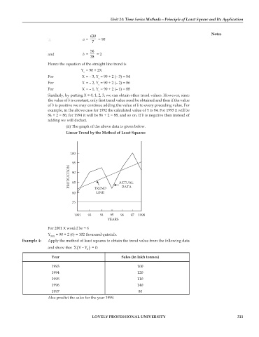
(ii) The graph of the above data is given below.
Linear Trend by the Method of Least Squares

100

95
PRODUCTION 90 ACTUAL

85

LINE
80 TREND DATA
75

1991 93 94 95 96 97 1998
YEARS
For 2001 X would be + 6
Y = 90 + 2 (6) = 102 thousand quintals.
2001
Example 4: Apply the method of least squares to obtain the trend value from the following data
)
∑
and show that ( − YY = 0:
c
Year Sales (in lakh tonnes)
1993 100
1994 120
1995 110
1996 140
1997 80
Also predict the sales for the year 1999.

LOVELY PROFESSIONAL UNIVERSITY 311