Page 313 - DECO504_STATISTICAL_METHODS_IN_ECONOMICS_ENGLISH

Statistical Methods in Economics

Notes ∑XlogY
log b = 2 ... (4)
∑X
With the values of a and b, the logarithmic straight line equation can now be written as
log Y = log a + X log b ... (5)
The property of b for a geometric straight line is of considerable significance. When it
has been converted into a pure percentage it defines the annual rate of growth or
decline of the series. Being an abstract measure, it allows comparison of trends all
described by straight lines on ratio paper, of series with different original units. Series,
such as production of all kinds, population or national income, become immediately
comparable, and conclusions about the direction and magnitude of economic activities
can be easily drawn. This measure provides an effective device for the study of the
socio-economic changes in a country.

Mathematical curves are useful to describe the general movement of a time series,
but it is doubtful whether any analytical significance should be attached to them,
except in special cases.

So far we have studied the method of fitting an arithmetic or geometric straight line
to a time series. But many time series are best described by curves, and not by straight
lines. In such situations, the linear model does not adequately describe the change in
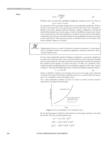
the variable as time changes. To study such cases, we often use a parabolic curve,
which is described mathematically by a second degree equation. Such a curve is given
in Figure 1. The general mathematical form of the second-degree parabolic trend is
Y= + X+ Xab c 2 ... (6)
where a is still the Y intercept, b is the slope of the curve at the origin, and c is the rate
of change in the slope. It should be noted that, just as b is a constant in the first-degree
curve c is a constant in the second-degree curve.
The c value determines whether the curve is concave or convex and the extent to
which the curve departs from linearity.

Unit of Measure Parabolic Curve

General Equation for
a parabolic Curve
2
Y= + bx + cx
a
Time
Figure 1: Form and Equation for a Parabolic Curve.
We use the least squares method to determine the second-degree equation to describe
the best fit. The three normal equations are
∑Y = na b ∑ + +X c ∑ X 2
∑XY = ∑ a ∑X + b 2 + c ∑ X X 2

2
∑XY = ∑ a 2 ∑X + b 3 + c ∑ X X 4

308 LOVELY PROFESSIONAL UNIVERSITY