Page 315 - DECO504_STATISTICAL_METHODS_IN_ECONOMICS_ENGLISH

Statistical Methods in Economics

Notes The trend values are obtained by substituting the X’s and X ’s into the trend equation.
2
These values have been given in the last column of Table 24.2.
Suppose we want to forecast India’s exports of engineering goods for the year 1989,
we observe that 1989 is 6 years ahead of the origin for the equation established above.
Thus, when this value of X (= 6), is substituted into the second degree equation, we
get
Y (1989) = 193.45 + 72.33 X + 15.98 X 2
cal
= 193.45 + 72.33 (6) + 15.98 (6) 2
= 1202.70
Based upon the past trend, we can conclude that India’s exports of engineering goods
during 1989 would be Rs. 1202.70 crores. This extra-ordinarily large forecast suggests,
however, that we must be more careful in forecasting with a parabolic curve than
when using a linear trend. The slope of the second degree equation is continually
increasing. Therefore, the parabolic curve may become a poor estimator as we attempt
to predict further into the future.
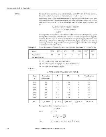
Example 3: Below are given the figures of production in (thousand quintals) of a sugar factory:
Year: 1992 1993 1994 1995 1996 1997 1998

Production 80 90 92 83 94 99 92
(in ‘000 quintals):

(i) Fit a straight line trend to these figures.
(ii) Plot these figures on a graph and show the trend line.
(iii) Estimate the production in 2001.
Solution:
(i) FITTING THE STRAIGHT LINE TREND

Year Production X XY X 2 Trend values
X (‘000 qtls.) Y Y
c
1992 80 – 3 – 240 9 84
1993 90 – 2 – 180 4 86
1994 92 – 1 – 92 1 88
1995 83 0 0 0 90
1996 94 + 1 + 94 1 92
1997 99 + 2 + 198 4 94
1998 92 + 3 + 276 9 96

2
N = 7 ∑ Y = 630 ∑ X = 0 ∑ XY = 56 ∑ X = 28 ∑ Y c = 630
The equation of the straight line trend is
Y = a + bX
c
Since ∑X = 0

∑Y ∑XY
a = , b = 2
N ∑X
Here ∑Y = 630, N = 7, ∑XY = 56, ∑X = 28,
2

310 LOVELY PROFESSIONAL UNIVERSITY