Page 311 - DECO504_STATISTICAL_METHODS_IN_ECONOMICS_ENGLISH

Statistical Methods in Economics

Notes Therefore, we can get

∑Y
a = ... (1)
n
∑XY
b = 2 ... (2)
∑X
From the above expressions, we can state that a, the value of Y at the origin, is the arithmetic mean of
the Y variable. The value of b, of course, is the average amount of change in the trend values per unit
of time.
It should be noted that in computing the trend it is convenient to use the middle of the series as the
origin. If the series contains an odd number of periods, the origin is the middle of the given period. If
an even number of periods is involved, the origin is set between the two middle periods.
It is important to recognize that the least squares technique requires that the type of line desired be
specified. Once this has been done, the technique generates the line of best fit of that type, that is, the
least squares line. Thus, for any set of data, one could generate: (a) a least squares straight line, (b) a
geometric least squares straight line, and (c) a least squares second-degree parabola. If one were to
compute each of the above and determine which of the three has the least sum of squared deviations,
the least squares criterion could also be used to indicate which type of line provides the best fit.
In case of a straight line trend, for any set of data, it is sufficient to compute ∑Y , ∑X , ∑XY , and

∑X 2 . We shall generate these values for the data in Example 1.
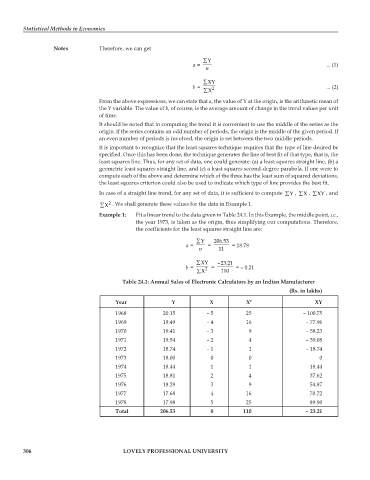
Example 1: Fit a linear trend to the data given in Table 24.1. In this Example, the middle point, i.e.,
the year 1973, is taken as the origin, thus simplifying our computations. Therefore,
the coefficients for the least squares straight line are:

∑Y 206.53
a = = = 18.78
n 11

∑XY –23.21
b = 2 = = – 0.21
∑X 110
Table 24.1: Annual Sales of Electronic Calculators by an Indian Manufacturer
(Rs. in lakhs)

Year Y X X 2 XY
1968 20.15 – 5 25 – 100.75
1969 19.49 – 4 16 – 77.96
1970 19.41 – 3 9 – 58.23
1971 19.54 – 2 4 – 39.08
1972 18.74 – 1 1 – 18.74
1973 18.00 0 0 0
1974 18.44 1 1 18.44
1975 18.81 2 4 37.62
1976 18.29 3 9 54.87
1977 17.68 4 16 70.72
1978 17.98 5 25 89.90
Total 206.53 0 110 – 23.21

306 LOVELY PROFESSIONAL UNIVERSITY