Page 391 - DECO504_STATISTICAL_METHODS_IN_ECONOMICS_ENGLISH

Statistical Methods in Economics

Notes x c = 75.115

Critical value
0.45 0.5
α = 0.05

z
z = – 1.645 =0

75.115 78 =80 (a)

= 0.8340
1–

0.1660
z = – 0.971 =0 (b)

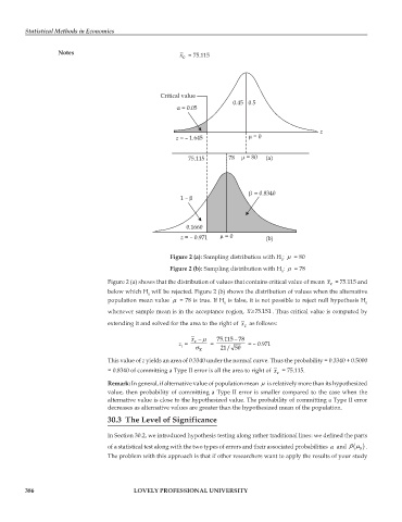
Figure 2 (a): Sampling distribution with H : μ = 80
0
Figure 2 (b): Sampling distribution with H : μ = 78
0
Figure 2 (a) shows that the distribution of values that contains critical value of mean x = 75.115 and
c
below which H will be rejected. Figure 2 (b) shows the distribution of values when the alternative
0
population mean value μ = 78 is true. If H is false, it is not possible to reject null hypothesis H
0 0
whenever sample mean is in the acceptance region, ≥75.151x . Thus critical value is computed by
extending it and solved for the area to the right of x as follows:
c
x − μ 75.115 − 78
z = c = = – 0.971
1 σ x 21/ 50
This value of z yields an area of 0.3340 under the normal curve. Thus the probability = 0.3340 + 0.5000
= 0.8340 of committing a Type II error is all the area to right of x = 75.115.
c
Remark: In general, if alternative value of population mean μ is relatively more than its hypothesized
value, then probability of committing a Type II error is smaller compared to the case when the
alternative value is close to the hypothesized value. The probability of committing a Type II error
decreases as alternative values are greater than the hypothesized mean of the population.
30.3 The Level of Significance

In Section 30.2, we introduced hypothesis testing along rather traditional lines: we defined the parts
βμ
of a statistical test along with the two types of errors and their associated probabilities α and ( ) .
a
The problem with this approach is that if other researchers want to apply the results of your study

386 LOVELY PROFESSIONAL UNIVERSITY