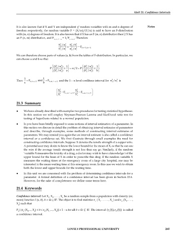
Page 293 - DMTH404_STATISTICS

Unit 21: Confidence Intervals

2
It is also known that if X and Y are independent  random variables with m and n degrees of Notes
freedom respectively, the random variable F = (X/m)/(Y/n) is said to have an F-distribution
with (m, n) degrees of freedom. It is also known that if X has an F (m, n) distribution then l/X has
an F (n, m) distribution, and F = 1/F . Therefore
m, n, 1 –  n, m, 
2
2
S / 2 2  S /S 2 1 ~ F
2
2


2
S / 2  2 / 2 (m 1),(n 1)
1 1 2 1
We can therefore choose paris of values (a, b) from the tables of F-distribution. In particular, we
can choose a and b so that
2
2
  (S / 2 ) 1    (S / 2 ) 1  
P
P  2 2 2 2     /2   2 2 2 2  
  (S / 1 ) a     (S / 1 ) b  
1
1
1 1
2
Then  F m,n, /2 and  F m,n,1 /2 and the 1 –  level confihnce interval for  2 / is

a b 2 1
 S 2 2 S 2 2 
 2  F n,m,1 /2 , 2  F n,m,1/ /2 

 S 1 S 1 
21.3 Summary
 We have already described with examples two procedures for testing statistical hypotheses.
In this section we will employ Neyman-Pearson Lamma and likelihood ratio test for
testing of hypothesis related to a normal population.
 In you have been briefly exposed to some notions of interval estimation of a parameter. In
this section we discuss in detail the problem of obtaining interval estimates of parameters
and describe, through examples, some methods of constructing interval extimates of
parameters. We may remind you again that an interval estimate is also called a confidence
interval or a confidence set. We first illustrate through small examples the need for
constructing confidence intervals. Suppose X denotes the tensile strength of a copper wire.
A potential user may desire to know the lower bound for the mean of X, so that he can use
the wire if the average tensile strength is not less than say go. Similarly, if the random
‘variable X measures the toxicity of a drug, a doctor may wish to have a knowledge t of the
upper bound for the hean of X in order to prescribe this dmg. If the random variable X
measures the waiting times at the emergency room of a large city hospital, one may be
interested in the mean waiting time at this emergency room. In this case we wish to obtain
both the lower and upper bounds for the waiting time.

 In this unit we are concerned with the problem of determining confidence intervals for a
parameter. A formal definition of a confidence interval has been given in Section 15.6.
However, for the sake of completeness we define some terms here.
21.4 Keywords

Confidence interval: Let X , X , . . . , X be a random sample from a population with density (or,
1 2 n
1
mass) function f (x, ),    R . The object is to find statistics r ( X . . . . . , X ) and r (X , . . . ,
L 1 n U 1
X ) such that
n
1
P { (r (X ,..., X )    r (X ,..., X )]  1 –  for all    C R . The interval (r (X),r (X)) is called
 L 1 n U 1 n L U
a confidence interval.

LOVELY PROFESSIONAL UNIVERSITY 285