Page 208 - DMGT404 RESEARCH_METHODOLOGY

Research Methodology

Notes There are two methodologies to anticipate future. They are called qualitative and quantitative.
But both start with the same premise, that an understanding of the future is predicted on an
understanding of the past and present environment. In this unit, we will mainly deal with
quantitative methods. We will also distinguish between forecast and prediction. We use the
word forecast when some logical method is used.
The quantitative decision maker always considers himself or herself accountable for a forecast—
within reason. Let us look at the conceptual model first and then the mathematical model and
algorithms in turn which are used for making forecast.

10.1 Time Series Analysis

Time has strange, fascinating and little understood properties. Virtually every process on earth
is determined by a time variable. One of the most frequently encountered managerial decision
situations involving forecasting is to measure the effect that time has on the sales of a product,
the market price of a security, the output of individuals, work shifts, companies, industries,
societies and so on. A fundamental conceptual model in all of these situations is the product life
cycle concept which goes through four stages – introduction, growth, maturity and decline. Let
us look at this concept in greater detail before we apply it.
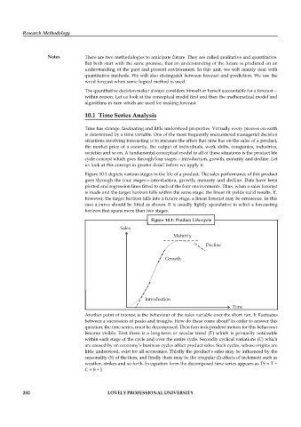
Figure 10.1 depicts various stages in the life of a product. The sales performance of this product
goes through the four stages—introduction, growth, maturity and decline. Data have been
plotted and regression lines fitted to each of the four environments. Thus, when a sales forecast
is made and the target horizon falls within the same stage, the linear fit yields valid results. If,
however, the target horizon falls into a future stage, a linear forecast may be erroneous. In this
case a curve should be fitted as shown. It is usually lightly speculative to select a forecasting
horizon that spans more than two stages.
Figure 10.1: Product Life-cycle
Sales
Maturity
Decline

Growth

Introduction
Time
Another point of interest is the behaviour of the sales variable over the short run. It fluctuates
between a succession of peaks and troughs. How do these come about? In order to answer this
question, the time series, must be decomposed. Then four independent motors for this behaviour
become visible. First there is a long-term or secular trend (T) which is primarily noticeable
within each stage of the cycle and over the entire cycle. Secondly cyclical variations (C) which
are caused by an economy’s business cycles affect product sales. Such cycles, whose origins are
little understood, exist for all economies. Thirdly the product’s sales may be influenced by the
seasonality (S) of the item, and finally there may be the irregular (I) effects of inclement such as
weather, strikes and so forth. In equation form the decomposed time series appears as TS = T +
C + S + I.

202 LOVELY PROFESSIONAL UNIVERSITY