Page 212 - DMGT404 RESEARCH_METHODOLOGY

Research Methodology

Notes Let us quantify this seasonality and illustrate how it may be used in a decision situation. There
are, as is often the case, a number of decision tools that may be applied. The reader may be
familiar with the term ratio-to-moving-average. It is a widely used method for constructing a
seasonal index and programs are available in most larger computer libraries. Usually the method
assumes a 12-period season like the twelve months of the year. There is a more efficient method
which yields good statistical results. It is especially helpful in manual calculations of the seasonal
index and when the number of seasonal periods is small like the four quarters of a year, the six
hours of a stock exchange trading day or the five days of a work week. This method is known as
simple average and will be used for illustration purposes.
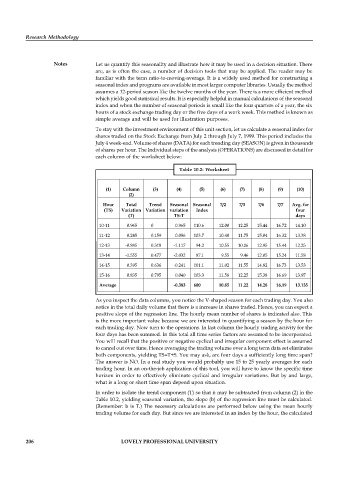
To stay with the investment environment of this unit section, let us calculate a seasonal index for
shares traded on the Stock Exchange from July 2 through July 7, 1999. This period includes the
July 4 week-end. Volume of shares (DATA) for each trending day (SEASON) is given in thousands
of shares per hour. The Individual steps of the analysis (OPERATIONS) are discussed in detail for
each column of the worksheet below:

Table 10.2: Worksheet

(1) Column (3) (4) (5) (6) (7) (8) (9) (10)
(2)
Hour Total Trend Seasonal Seasonal 7/2 7/3 7/6 7/7 Avg. for
(TS) Variation Variation variation Index four
(T) TS-T days
10-11 0.965 0 0.965 110.6 12.00 12.25 15.44 16.72 14.10
11-12 0.245 0.159 0.086 103.7 10.40 11.75 15.04 16.32 13.38
12-13 -0.885 0.318 -1.117 94.2 10.55 10.06 12.95 15.44 12.25

13-14 -1.555 0.477 -2.032 87.1 9.55 9.46 12.05 15.24 11.58
14-15 0.395 0.636 -0.241 101.1 11.02 11.55 14.82 16.73 13.53
15-16 0.835 0.795 0.040 103.3 11.58 12.25 15.38 16.69 13.97
Average -0.383 600 10.85 11.22 14.28 16.19 13.135

As you inspect the data columns, you notice the V-shaped season for each trading day. You also
notice in the total daily volume that there is a increase in shares traded. Hence, you can expect a
positive slope of the regression line. The hourly mean number of shares is indicated also. This
is the more important value because we are interested in quantifying a season by the hour for
each trading day. Now turn to the operations. In last column the hourly trading activity for the
four days has been summed. In this total all time series factors are assumed to be incorporated.
You will recall that the positive or negative cyclical and irregular component effect is assumed
to cancel out over time. Hence averaging the trading volume over a long term data set eliminates
both components, yielding TS=T+S. You may ask, are four days a sufficiently long time span?
The answer is NO. In a real study you would probably use 15 to 25 yearly averages for each
trading hour. In an on-the-job application of this tool, you will have to know the specific time
horizon in order to effectively eliminate cyclical and irregular variations. But by and large,
what is a long or short time span depend upon situation.

In order to isolate the trend component (T) so that it may be subtracted from column (2) in the
Table 10.2, yielding seasonal variation, the slope (b) of the regression line must be calculated.
(Remember: b is T.) The necessary calculations are performed below using the mean hourly
trading volume for each day. But since we are interested in an index by the hour, the calculated

206 LOVELY PROFESSIONAL UNIVERSITY