Page 209 - DMGT404 RESEARCH_METHODOLOGY
P. 209
Unit 10: Time Series


          This creates a complex situation in time series analysis. Each factor must be quantified and its  Notes
          effect ascertained upon product sales. Let us see how this is done. The long-term trend effect T is
          reflected in the slope b of the regression equation. We already know how b is calculated even
          though minor modifications of the decision formulas will be encountered soon. The quantification
          of the cyclical component C is beyond the scope of this book. However, since business cycles
          always proceed from peak to trough to new peak and so on, their positive and negative effects
          upon a product’s sales cancel out in the long-run. Hence in managerial, as opposed to economic,
          decision making, the sum effect of the business cycles may be set equal to zero. This eliminates
          the C factor from the equation. Seasonality, if present, is something that must be taken into
          consideration because it is a product-inherent variable and therefore it is under the immediate
          control of the decision maker. We will quantify the S component and keep it in the equation.
          Finally, there are the irregular variations. Do we know in July whether the weather will be
          sunny and mild during the four  weeks before  Diwali? We  don’t, but  we know  that if  this
          happens, Diwali  sales will  be severely  impacted. Can  we  forecast  such  horrible  weather
          conditions? Not really. We cannot forecast them because they cannot be quantified—a rather
          unpleasant characteristic  they share with all other type of irregular  variations like  strikes,
          earthquakes, power failure, etc. Yet, something strange usually happens after such an irregular
          variation from “normal” has  occurred. Whatever people did  not do  because of  it, like not
          buying a product, they attempt to catch up with quickly. Therefore the factor effect may also be
          assumed to cancel out over time and it may be dropped from the equation which then appears
          to the manager as TS = T + S.

          Linear Analysis

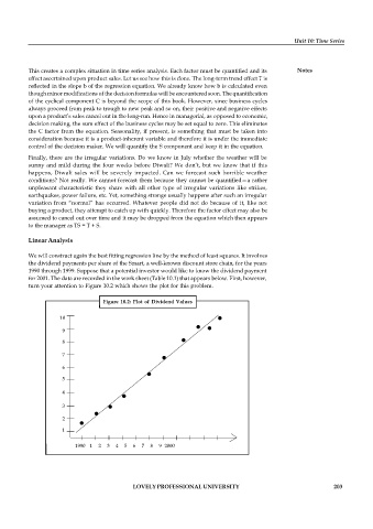
          We will construct again the best fitting regression line by the method of least squares. It involves
          the dividend payments per share of the Smart, a well-known discount store chain, for the years
          1990 through 1999. Suppose that a potential investor would like to know the dividend payment
          for 2001. The data are recorded in the work sheet (Table 10.1) that appears below. First, however,
          turn your attention to Figure 10.2 which shows the plot for this problem.


                                  Figure  10.2: Plot  of Dividend  Values

                    10
                     9

                     8
                     7

                     6
                     5

                     4
                     3

                     2
                     1

                         1990   1    2    3    4    5    6    7    8    9  2000


                                           LOVELY PROFESSIONAL UNIVERSITY                                   203

