Page 265 - DMGT501_OPERATIONS_MANAGEMENT

Unit 11: Inventory Model

Since in most cases demand is probabilistic, in such cases policies are based on expected costs Notes
rather than actual costs. Expected costs are obtained by multiplying the actual costs for a particular
occurrence with the probability of the occurrence of the event. This type of model is called the
‘Christmas tree problem’.
In the cases of discrete probabilities, the manner in which frequency distributions can be used

to decide on order quantities is explained with this example. Say, a television dealer finds that
cost of holding a television in stock for a week is 30 and the cost of unit shortage is 70. For one
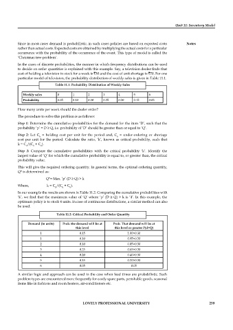
particular model of television, the probability distribution of weekly sales is given in Table 11.1.
Table 11.1: Probability Distribution of Weekly Sales

Weekly sales 0 1 2 3 4 5 6
Probability 0.05 0.10 0.20 0.25 0.20 0.15 0.05
How many units per week should the dealer order?

The procedure to solve this problem is as follows:
Step 1: Determine the cumulative probabilities for the demand for the item ‘D’, such that the
probability ‘p’ = D ≥ Q, i.e. probability of ‘D’ should be greater than or equal to ‘Q’.
Step 2: Let C = holding cost per unit for the period and, C = under-ordering or shortage
h b
cost per unit for the period. Calculate the ratio, ‘k’, known as critical probability, such that
k = C /(C + C ).
h h b
Step 3: Compare the cumulative probabilities with the critical probability ‘k’. Identify the
largest value of ‘Q’ for which the cumulative probability is equal to, or greater than, the critical
probability value.
This will give the required ordering quantity. In general terms, the optimal ordering quantity,
Q* is determined as:
Q*= Max. ‘p’ (D ≥ Q) > k

Where, k = C /(C + C ).
h h b
In our example the results are shown in Table 11.2. Comparing the cumulative probabilities with
‘k’, we find that the maximum value of ‘Q’ where ‘p’ (D ≥ Q) > k is ‘4’. In this example, the

optimum policy is to stock 4 units. In case of continuous distributions, a similar method can also
be used.

Table 11.2: Critical Probability and Order Quantity

Demand (in units) Prob. the demand will be at Prob. That demand will be at
this level this level or greater P(d>Q)
1 0.15 1.00>0.30
1 0.10 0.95>0.30
2 0.10 0.85>0.30
3 0.25 0.65>0.30
4 0.20 0.40>0.30
5 0.15 0.20>0.30
6 0.05 0.05

A similar logic and approach can be used in the case when lead times are probabilistic. Such
problem types are encountered more frequently for costly spare parts, perishable goods, seasonal
items like in fashions and room heaters, air-conditioners etc.

LOVELY PROFESSIONAL UNIVERSITY 259