Page 126 - DECO504_STATISTICAL_METHODS_IN_ECONOMICS_ENGLISH

Statistical Methods in Economics

Notes ∑ fd
X = A + = 25 + 0 = 25
∑ f 100
Mode (Z) is located in the class interval 20–30.
f − f 27 23
−
l + 1 0 i × = 20 + × 10
Z= 1
2 f − 1 f − 0 f 2 227 − 23 21
−
×
4
= 20 + × 10 = 20 + 4 = 24
10
∑ fd 2 ⎛ ∑ fd ⎞ 2 16000 ⎛ 0 ⎞ 2
σ = − ⎜ ⎟ = − ⎜ ⎟
N ⎝ N ⎠ 100 ⎝ 100 ⎠

= 160 = 12.65 Approx.
−
X – Z 25 24 1
Coefficient of Skewness = = = = 0.08
σ 12.65 12.65
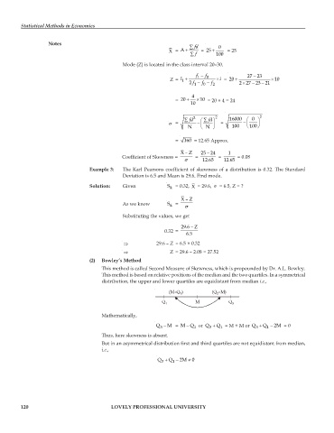
Example 3: The Karl Pearsons coefficient of skewness of a distribution is 0.32. The Standard
Deviation is 6.5 and Mean is 29.6. Find mode.
Solution: Given S k = 0.32, X = 29.6, σ = 6.5, Z = ?

X – Z
As we know S k = σ

Substituting the values, we get
−
29.6 Z
0.32 = 6.5
⇒ 29.6 – Z = 6.5 × 0.32
⇒ Z = 29.6 – 2.08 = 27.52
(2) Bowley’s Method
This method is called Second Measure of Skewness, which is propounded by Dr. A.L. Bowley.
This method is based on relative positions of the median and the two quartiles. In a symmetrical
distribution, the upper and lower quartiles are equidistant from median i.e.,
(M–Q ) (Q –M)
1
2
Q 1 M Q 3

Mathematically,
−
Q − M = MQ or Q + Q = M + M or Q + 3 Q − 1 2M = 0
3
1
1
3
Thus, here skewness is absent.
But in an asymmetrical distribution first and third quartiles are not equidistant from median,
i.e.,
Q + 3 Q − 1 2M ≠ 0

120 LOVELY PROFESSIONAL UNIVERSITY