Page 284 - DECO504_STATISTICAL_METHODS_IN_ECONOMICS_ENGLISH

Statistical Methods in Economics

Notes Trends can be linear, or they can be curvilinear, i.e., parabola. A straight line has a constant rate of
change, while a parabola represents a changing rate of change. In fact, parabola shows a trend that is
increasing at an increasing rate. The decision as to whether the trend should be a straight line or a
parabola is an important one. It certainly is a subjective matter, and one has to be careful to choose
the right trend to represent the data. Once the decision is made to the implied nature of the trend
(linear or non-linear), one computes the rate of change and any errors in the choice of the trend curve
will affect the results. Computation of the rate of change and measuring the trend is a process known
as “fitting a curve to the data”.
Before we discuss curve fitting, however, let us first consider the general types of trends that are
available to represent the data. We shall identify three types of trends which are very popular in the
analysis:
The Linear Trend (Straight Line, Constant Rate of Change)

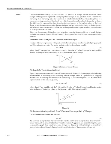
This type of trend is represented in Figure 2, which shows two linear trend curves, (1) sloping upwards
and (2) sloping downwards. The mathe-matical model for these linear trend is
Y = a + bX ... (1)
where X and Y are variables, a is the Y-intercept (i.e., the value of Y when X is equal to zero), and b is
the rate of change of Y for unit change in X, or the constant rate of change.

1( )
x
(1)

(2)
x
Figure 2: Pattern of Linear Trend.
The Parabolic Trend (Changing Rate)

Figure 3 represents the pattern of this trend. In this pattern (1) the trend is slopping upwards, indicating
that the trend is increasing at an increasing rate of change, while in (2) the trend is slopping
downwards, indicating that the trend is increasing at a decreasing rate. The mathematical
representation of this curve is given by

Y = ab+ X+ X 2 ... (2)
c
where X and Y are variables, a is the Y-intercept (or the value of Y when X is zero), and b and c are the
rates of change of Y at given values of X which vary with different values of X.

1( )
x
(1)
(2)

x
(0, 0)

Figure 3:
The Exponential or Logarithmic Trend (Constant Percentage Rate of Change)
The mathematical model for this curve is:

Y = ab x ... (3)
It is known as an exponential curve because the variable X appears as an exponent in the expression—
unlike the other two cases stated earlier, where the variable X appeared as a factor. Plotting this curve
on a semi-log graph sheet would produce a straight line (Figure 4), while plotting it on an ordinary
graph sheet produces Figure 5. Taking logarithms of both sides of the expression (3), we get

278 LOVELY PROFESSIONAL UNIVERSITY