Page 286 - DECO504_STATISTICAL_METHODS_IN_ECONOMICS_ENGLISH

Statistical Methods in Economics

Notes In a time series of annual data, only the secular trend, cyclical and irregular components are considered
since the seasonal variation makes a complete, regular cycle within each year and thus do not affect
the annual data. As secular trend can be described by a trend line, it is possible to isolate the remaining,
cyclical and irregular components from the trend. For simplicity, we shall assume that the cyclical
component explains most of the variations left unexplained by the trend component. However, in
situations where this assumption does not hold good, methods such as Fourier analysis and spectral
analysis can be used to analyse cyclical component in a time series. (These advanced techniques are
beyond the scope of this text.)
If we use a time series composed of annual data, we can find the fraction of the trend by dividing the
Y
original value (Y) by the corresponding trend value ( cal ) for each observation in the time series.
We then take the percentage of this value by multiplying by 100. This gives us the measure of cyclical
variation as a per cent of trend. Mathematically, this can be expressed as:
Y
Per cent of trend = Y cal × 100 ... (5)

where Y is the actual observation of the time series data, and Y cal is the calculated trend value in the
time series.
The above procedure used to identify cyclical variation is called the residual method.
Example 1: Let us consider the data given in Table 1 which refers to the yield per hectare of a
certain foodgrain in an Indian state during 1970 to 1978. The third column in this
table refers to the values of linear trend for each time period. The trend line has been
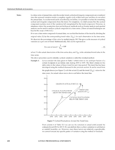
developed using the method discussed in the previous section. It can be noted from
Y
the graph drawn (see Figure 7) with the actual (Y) and the trend ( cal ) values for the
nine years, the actual values move above and below the trend line.
Y
19.4

19.0 GRAPH OF ACTUAL POINT (Y)

TREND LINE
18.6 CYCLICAL FLUCTUATIONS
cal
ABOVE THE TREND LINE (GRAPH OF Y )
18.2
CYCLICAL FLUCTUATIONS
BELOW THE TREND LINE
17.8

17.4

17.0
1970 1971 1972 1973 1974 1975 1976 1977 1978
Figure 7: Cyclical Fluctuations Around the Trend Line.

From column 4 of Table 22.1 we can see the variation in actual yield around the
estimated trend (98.8 to 101.7). We can attribute these cyclical variations to such factors
as rainfall, humidity, etc. However, since these factors are relatively unpredictable,
we cannot forecast any specific patten of variation using the method of residuals.

280 LOVELY PROFESSIONAL UNIVERSITY