Page 197 - DMTH404_STATISTICS

Unit 14: Theoretical Probability Distributions

a city per week, the number of defects per meter of cloth, the number of insurance claims per Notes
year, the number breakdowns of machines at a factory per day, the number of arrivals of
customers at a shop per hour, the number of typing errors per page etc.
14.6.1 Poisson Process

Let us assume that on an average 3 telephone calls are received per 10 minutes at a telephone
exchange desk and we want to find the probability of receiving a telephone call in the next 10
minutes. In an effort to apply binomial distribution, we can divide the interval of 10 minutes
into 10 intervals of 1 minute each so that the probability of receiving a telephone call (i.e., a
success) in each minute (i.e., trial) becomes 3/10 ( note that p = m/n, where m denotes mean).
Thus, there are 10 trials which are independent, each with probability of success = 3/10. However,
the main difficulty with this formulation is that, strictly speaking, these trials are not Bernoulli
trials. One essential requirement of such trials, that each trial must result into one of the two
possible outcomes, is violated here. In the above example, a trial, i.e. an interval of one minute,
may result into 0, 1, 2, ...... successes depending upon whether the exchange desk receives none,
one, two, ...... telephone calls respectively.
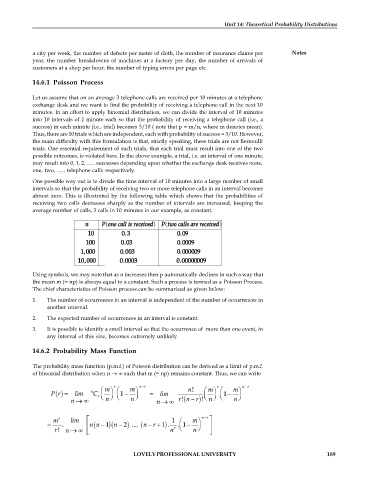
One possible way out is to divide the time interval of 10 minutes into a large number of small
intervals so that the probability of receiving two or more telephone calls in an interval becomes
almost zero. This is illustrated by the following table which shows that the probabilities of
receiving two calls decreases sharply as the number of intervals are increased, keeping the
average number of calls, 3 calls in 10 minutes in our example, as constant.
a
P one call is receivedf P two calls are receivedf
a
n
10 0.3 0.09
100 0.03 0.0009
1,000 0.003 0.000009
10,000 0.0003 0.00000009

Using symbols, we may note that as n increases then p automatically declines in such a way that
the mean m (= np) is always equal to a constant. Such a process is termed as a Poisson Process.
The chief characteristics of Poisson process can be summarised as given below:
1. The number of occurrences in an interval is independent of the number of occurrences in
another interval.
2. The expected number of occurrences in an interval is constant.
3. It is possible to identify a small interval so that the occurrence of more than one event, in
any interval of this size, becomes extremely unlikely.

14.6.2 Probability Mass Function

The probability mass function (p.m.f.) of Poisson distribution can be derived as a limit of p.m.f.
of binomial distribution when n   such that m (= np) remains constant. Thus, we can write

r n r ! n r n r

n
P ( ) r = lim C r ç æ mö æ 1 mö lim= æ ç mö æ 1 mö ÷
÷ ç
÷
÷ ç
)! n ø è

n   è n ø è n ø n   ( ! r n r è n ø

m r lim é 1 æ mö n r ù
. 1
= . ( n n  1 )(n  ) 2 .... (n r + ) 1 . r ç ÷ ú
ê
! r n   ê ë n è n ø ú û
LOVELY PROFESSIONAL UNIVERSITY 189