Page 213 - DMTH404_STATISTICS

Unit 15: Exponential Distribution and Normal Distribution

15.3.2 Probability Density Function Notes

If X is a continuous random variable, distributed normally with mean m and standard deviation
, then its p.d.f. is given by

2
1 X m- ö
1 - ç æ ÷
p X .e 2 è  ø where - ¥ < X < ¥.
( ) =
 2p
Here p and e are absolute constants with values 3.14159.... and 2.71828.... respectively.
It may be noted here that this distribution is completely known if the values of mean m and
standard deviation s are known. Thus, the distribution has two parameters, viz. mean and
standard deviation.

15.3.3 Shape of Normal Probability Curve

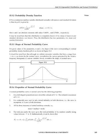
For given values of the parameters, m and s, the shape of the curve corresponding to normal
probability density function p(X) is as shown in Figure 15.2
It should be noted here that although we seldom encounter variables that have a range from
- ¥ to ¥, as shown by the normal curve, nevertheless the curves generated by the relative
frequency histograms of various variables closely resembles the shape of normal curve.

Figure 15.2

15.3.4 Properties of Normal Probability Curve

A normal probability curve or normal curve has the following properties:

1. It is a bell shaped symmetrical curve about the ordinate at X = m . The ordinate is maximum
at X = m .
2. It is unimodal curve and its tails extend infinitely in both directions, i.e., the curve is
asymptotic to X axis in both directions.
3. All the three measures of central tendency coincide, i.e.,
mean = median = mode

4. The total area under the curve gives the total probability of the random variable taking
values between - ¥ to ¥. Mathematically, it can be shown that

2
1 X m- ö
¥ ¥ 1 - ç æ ÷
P (- ¥ < X < ¥ ) = -¥ ò p X -¥ ò  2p e 2 è  ø dX = 1.
( )dX =

LOVELY PROFESSIONAL UNIVERSITY 205