Page 216 - DMTH404_STATISTICS

Statistics

Notes of the distribution of z are fixed, it is a known distribution and is termed as standard normal
distribution (s.n.d.). Further, z is termed as a standard normal variate (s.n.v.).
It is obvious from the above that the distribution of any normal variate X can always be transformed
into the distribution of standard normal variate z. This fact can be utilised to evaluate the
integral given above.

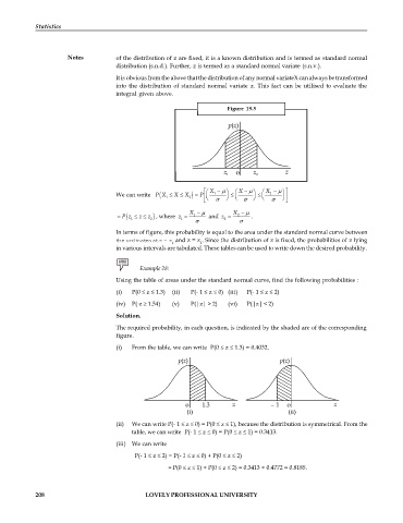
Figure 19.5

m
m ù
m
éæ X - ö æ X - ö æ X - ö
P
We can write (X £ X £ X 2 ) P= ç ê 1 ÷ £ ç ÷ £ ç 2 ÷ ú
1
ë è  ø è  ø è  ø û
X - m X - m
= P z £ £ z 2 ) , where z = 1 and z = 2 .
z
( 1
2
1
 
In terms of figure, this probability is equal to the area under the standard normal curve between
the ordinates at z = z and z = z . Since the distribution of z is fixed, the probabilities of z lying
1 2
in various intervals are tabulated. These tables can be used to write down the desired probability.
Example 28:
Using the table of areas under the standard normal curve, find the following probabilities :
(i) P(0 £ z £ 1.3) (ii) P(- 1 £ z £ 0) (iii) P(- 1 £ z £ 2)
(iv) P( z  1.54) (v) P(|z| > 2) (vi) P(|z| < 2)
Solution.

The required probability, in each question, is indicated by the shaded are of the corresponding
figure.
(i) From the table, we can write P(0 £ z £ 1.3) = 0.4032.

(ii) We can write P(- 1 £ z £ 0) = P(0 £ z £ 1), because the distribution is symmetrical. From the
table, we can write P(- 1 £ z £ 0) = P(0 £ z £ 1) = 0.3413.

(iii) We can write
P(- 1 £ z £ 2) = P(- 1 £ z £ 0) + P(0 £ z £ 2)
= P(0 £ z £ 1) + P(0 £ z £ 2) = 0.3413 + 0.4772 = 0.8185.

208 LOVELY PROFESSIONAL UNIVERSITY