Page 278 - DCOM504_SECURITY_ANALYSIS_AND_PORTFOLIO_MANAGEMENT

Unit 11: Capital Market Theory

The extent of this movement determines the price you are willing to pay (alternately, the return Notes
you demand) for holding asset A. The lower the average correlation A has with the rest of the
assets in the portfolio, the more the frontier, and hence T, will move to the left. This is good news
for the investor – if A moves your portfolio left, you will demand lower expected return because
it improves your portfolio risk-return profile. This is why the CAPM is called the “Capital Asset
Pricing Model.” It explains relative security prices in terms of a security’s contribution to the
risk of the whole portfolio, not its individual standard deviation.
The CAPM is a theoretical solution to the identity of the tangency portfolio. It uses some ideal
assumptions about the economy to argue that the capital weighted world wealth portfolio is the
tangency portfolio, and that every investor will hold this same portfolio of risky assets. Even
though it is clear they do not, the CAPM is still a very useful tool. It has been taken as a
prescription for the investment portfolio, as well as a tool for estimating an expected rate of
return.

11.3 Further Explorations of the Capital Asset Pricing Model

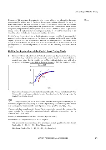
1. Risk-return Trade-off: A Technical Aside: Recall from last unit that, when investors are well
diversified, they evaluate the attractiveness of a security based upon its contribution to
portfolio risk, rather than its volatility per se. The intuition is that an asset with a low
correlation to the tangency portfolio is desirable, because it shifts the frontier to the left.
Figure 11.3

Stephen Ross formalized this institution in an article called Finance, published in The New
Palgrave. It is a simple argument that shows the theoretical basis for the ‘pricing’ part of the
Capital Asset Pricing Model.

Example: Suppose you are an investor who holds the market portfolio M and you are
considering the purchase of a quantity dx of asset A, by financing it via borrowing at the riskless
rate. This augments the return of the market portfolio by the quantity: dE = [E – R ]dx
m A f
Where d symbolizes a small quantity change. This investment also augments the variance of the
market portfolio. The variance of the market portfolio after adding the new asset is: v + dv = v
+ 2dx cov(A,m) + (dx) var(a)
2
2
The change in the variance is then: dv = 2 dx cov(A,m) + (dx) var(A)
For small dx’s this is approximately: dv = 2 dx cov(A,m)
This gives us the risk-return trade-off to investing in a small quantity of A: Risk-Return
Trade-off for A = dE /dv = [E – R ]dx/2 dx cov(A,m)
m A f
Risk-Return Trade-off for A = dE /dv = [E – R ]/2 cov(A,m)
m A f

LOVELY PROFESSIONAL UNIVERSITY 273