Page 282 - DCOM504_SECURITY_ANALYSIS_AND_PORTFOLIO_MANAGEMENT

Unit 11: Capital Market Theory

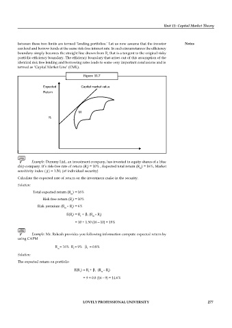
between these two limits are termed ‘lending portfolios.’ Let us now assume that the investor Notes
can lend and borrow funds at the same risk-free interest rate. In such circumstances the efficiency
boundary simply becomes the straight line drawn from R that is a tangent to the original risky
f
portfolio efficiency boundary. The efficiency boundary that arises out of this assumption of the
identical risk free lending and borrowing rates leads to some very important conclusions and is
termed as ‘Capital Market Line’ (CML).

Figure 11.7

Expected Capital market value
Return

M
R f

Example: Dummy Ltd., an investment company, has invested in equity shares of a blue
chip company. It’s risk-free rate of return (R ) = 10% , Expected total return (R ) = 16%, Market
f m
sensitivity index ( ) = 1.50, (of individual security)
Calculate the expected rate of return on the investment make in the security.
Solution:
Total expected return (R ) = 16%
m
Risk free return (R ) = 10%
f
Risk premium (R – R ) = 6%
m f
E(R) = R + i (R – R )
i f m f
= 10 + 1.50 (16 – 10) = 19%

Example: Mr. Rakesh provides you following information compute expected return by
using CAPM

R = 16% R = 9% i = 0.8%
m f
Solution:

The expected return on portfolio
E(R ) = R + i (R – R )
1 f m f
= 9 + 0.8 (16 – 9) = 14.6%

LOVELY PROFESSIONAL UNIVERSITY 277