Page 264 - DECO401_MICROECONOMIC_THEORY_ENGLISH

Unit-13: Theory of Monopoly Firm

monopolist will sell less quantity of the product (u) of OA units at more price OP in market A. On the Notes
1
other hand, he will sell more quantity ‘OB’ units at less price OP in market B. Marginal revenue of the
2
combined production of OQ units where combined marginal revenue is equal to marginal cost should
be equal in both the markets as it should be equal to marginal cost of the entire production which means

MR = MR = MR = MC
A B A+B

Suppose if this condition will not be satisfied, if in market A in comparison to market B, MR is less, then
it will be beneficial for discriminating monopolist to sell same units of market A to market B where he
will gain greater marginal revenue. This activity will go on till the marginal revenue of both markets
will be equal.

3. Price Determination

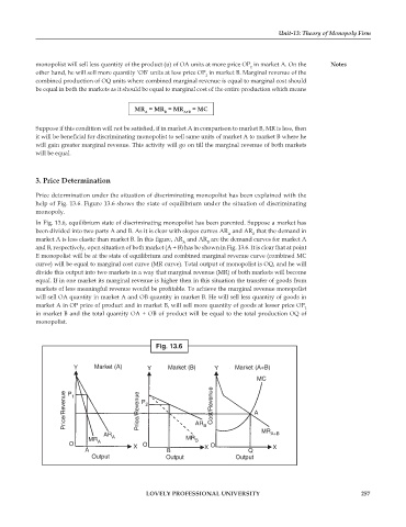
Price determination under the situation of discriminating monopolist has been explained with the
help of Fig. 13.6. Figure 13.6 shows the state of equilibrium under the situation of discriminating
monopoly.
In Fig. 13.6, equilibrium state of discriminating monopolist has been parented. Suppose a market has
been divided into two parts A and B. As it is clear with slopes curves AR and AR that the demand in
B
A
market A is less elastic than market B. In this figure, AR and AR are the demand curves for market A
A B
and B, respectively, open situation of both market (A + B) has be shown in Fig. 13.6. It is clear that at point
E monopolist will be at the state of equilibrium and combined marginal revenue curve (combined MC
curve) will be equal to marginal cost curve (MR curve). Total output of monopolist is OQ, and he will
divide this output into two markets in a way that marginal revenue (MR) of both markets will become
equal. If in one market its marginal revenue is higher then in this situation the transfer of goods from
markets of less meaningful revenue would be profitable. To achieve the marginal revenue monopolist
will sell OA quantity in market A and OB quantity in market B. He will sell less quantity of goods in
market A in OP price of product and in market B, will sell more quantity of goods at lesser price OP
2
in market B and the total quantity OA + OB of product will be equal to the total production OQ of
monopolist.

Fig. 13.6

Y Market (A) Y Market (B) Y Market (A+B)
MC
Price/Revenue 1 Price/Revenue P 2 Cost/Revenue A
P

AR A AR B MR A+B
MR A MR B
O X O O
A B X Q X
Output Output Output

LOVELY PROFESSIONAL UNIVERSITY 257