Page 250 - DMGT501_OPERATIONS_MANAGEMENT

Operations Management

Notes value. This means, l = m = n = 1. However, the estimate of demand turns out to be 50 per cent
higher than the true demand, i.e., ‘k = 1.5’.
Now putting these values into the equation, we can find the ratio of actual cost to “true” cost for

this case.
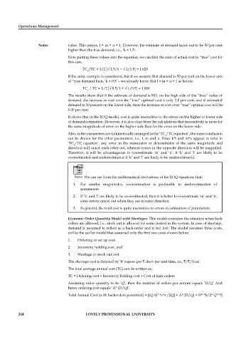
TC /TC = 1/2 [√ 1.5/1 + √ 1/1.5] = 1.020
e
If the same example is considered, but if we assume that demand is 50 per cent on the lower side
of “true demand then, ‘k = 0.5’ – we already know that l = m = n = 1 as before:

TC / TC = 1/2 [√ 0.5/1 + √ 1/0.5] = 1.060
e
The results show that if the estimate of demand is 50% on the high side of the “true” value of
demand, the increase in cost over the “true” optimal cost is only 2.0 per cent; and if estimated
demand is 50 percent on the lower side, then the increase in cost over “true” optimal cost will be
6.00 per cent.

It shows that in the EOQ model, cost is quite insensitive to the errors on the higher or lower side
of demand estimation. However, it is also clear from the calculations that insensitivity is more for
the same magnitude of error on the higher side than for the error on the lower side.

Also, as the parameters are symmetrically arranged in the ‘TC /TC equation’, the same conclusion
e
can be drawn for the other parameters, i.e., l, m and n. Since k*l and m*n appear in ratio in
‘TC /TC equation’, any error in the numerator or denominator of the same magnitude and
e

direction will cancel each other out, whereas errors in the opposite direction will be magnified.
Therefore, it will be advantageous to overestimate ‘m’ and ‘n’, if ‘k’ and ‘l’ are likely to be
overestimated and underestimated if ‘k’ and ‘l’ are likely to be underestimated.

We can see from the mathematical derivations of the EOQ equations that:
1. For similar magnitudes, overestimation is preferable to underestimation of
parameters.
2. If ‘k’ and ‘l’ are likely to be overestimated, then it is better to overestimate ‘m’ and ‘n’,
since errors cancel out when they are in same direction.

3. In general, the total cost is quite insensitive to errors in estimation of parameters.

Economic Order Quantity Model with Shortages: This model considers the situation when back
orders are allowed, i.e., stock out is allowed for some period in the system. In case of shortage,

demand is assumed to reflect as a back-order and is not lost. The model assumes three costs,

unlike the earlier model that assumed only the first two costs shown below:
1. Ordering or set up cost,
2. Inventory holding cost, and
3. Shortage or stock out cost.
The shortage cost is denoted by ‘b’ rupees per short per unit time, i.e., / /Year.
The total average annual cost (TC) can be written as,
TC = Ordering cost + Inventory holding cost + Cost of back orders

Assuming order quantity to be ‘Q’, then the number of orders per annum equals ‘D/Q’ And
hence ordering cost equals ‘A* (D/Q)’.
2
2
Total Annual Cost (with backorders permitted) = [(Q-S) *v*r /2Q] + A* (D/Q) + S* *b/2* Q EOQ ]

244 LOVELY PROFESSIONAL UNIVERSITY