Page 257 - DMGT501_OPERATIONS_MANAGEMENT

Unit 10: Economic Order Quantity

item cost varies with volume ordered, the result is a modified simple lot size situation called the Notes
quantity volume case or price break model.
The model assumes a discrete or step change rather than a per-unit change. For example, a Classic
cigarette sold from an open packet will cost 3.50 each. If purchased as a packet of 20, it would
cost 65.00. However, if you buy a carton of 10 packets it will only cost 600.00. To determine the
optimal quantity of cigarettes you want to buy, the model simply solves for the economic order
quantity for each price and at the point of price change.
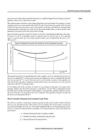
Figure 10.8 represents this concept. For 3 items, A, B, and C, a manufacturer offers price discounts.
For items ‘A’ and ‘B’ at quantities equal to or greater than ‘Q ’ and for item ‘C’ for a quantity
1

equal to or greater than ‘Q ’. The average annual variable costs are reflected by the curves ‘AA’,
2
‘BB’ and ‘CC’.
Figure 10.8: Quantity Discounts: Price Breaks are Given at Quantities Q and Q
1 2

The general procedure for determining the order quantity starts by checking the lowest cost
curve for an optimal Q EOQ . If that is unsuccessful, each higher cost curve is systematically checked
until the optimal Q EOQ is found. The total cost for each feasible economic order quantity and
price-break order quantity is tabulated, and the Q that leads to the minimum cost is the optimal
order size or the Q EOQ for the given item.
If the holding costs of the company are based on a percentage of unit prices, the largest order
quantity, which is also the lowest unit price, is solved first. The Q EOQ that is determined should

be valid. If it is not, the next-largest order quantity is examined till a feasible solution is found.
The cost of this Q EOQ is compared to the cost of using the order quantity at the price break, and
the lowest cost determines the Q EOQ .

10.2.2 Variable Demand and Constant Lead Time

We will now examine a moderately complex quantity/reorder point model in which lead time
does not vary, but demand does. This model is shown in Figure 10.9. In this model, we take into
account the possibility of a stock out. The model establishes buffer stocks that adequately protect
service to customers when demand is uncertain. The notations that are used in the model are
given below:
μ = Demand during lead time, a random variable
σ = Standard deviation of demand during lead time
u
μ¯ = Expected demand during lead time

LOVELY PROFESSIONAL UNIVERSITY 251