Page 258 - DMGT501_OPERATIONS_MANAGEMENT

Operations Management

Notes d¯ = Expected average daily demand
σ = Standard deviation of expected daily demand
d
D¯ = Expected annual demand
B = Buffer stock

z = Number of standard deviations needed for a specified confidence level
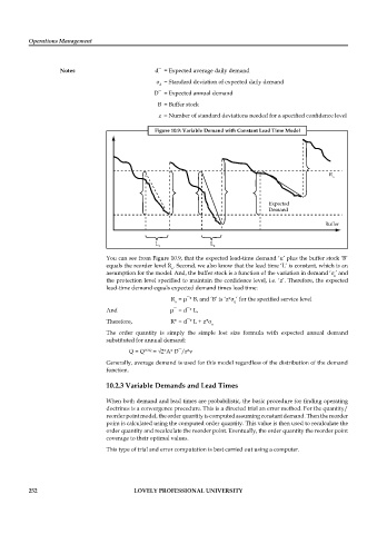
Figure 10.9: Variable Demand with Constant Lead Time Model

You can see from Figure 10.9, that the expected lead-time demand ‘u’ plus the buffer stock ‘B’
equals the reorder level R . Second, we also know that the lead time ‘L’ is constant, which is an
o
assumption for the model. And, the buffer stock is a function of the variation in demand ‘σ ’ and
u

the protection level specified to maintain the confidence level, i.e. ‘z’. Therefore, the expected

lead-time demand equals expected demand times lead time:

R = μ¯* B, and ‘B’ is ‘z*σ ’ for the specified service level
o u
And μ¯ = d¯* L,
Therefore, R* = d¯* L + z*σ
u
The order quantity is simply the simple lost size formula with expected annual demand
substituted for annual demand:
Q = Q EOQ = √2*A* D¯/r*v
Generally, average demand is used for this model regardless of the distribution of the demand
function.

10.2.3 Variable Demands and Lead Times

When both demand and lead times are probabilistic, the basic procedure for finding operating

doctrines is a convergence procedure. This is a directed trial an error method. For the quantity/
reorder point model, the order quantity is computed assuming constant demand. Then the reorder
point is calculated using the computed order quantity. This value is then used to recalculate the
order quantity and recalculate the reorder point. Eventually, the order quantity the reorder point
coverage to their optimal values.
This type of trial and error computation is best carried out using a computer.

252 LOVELY PROFESSIONAL UNIVERSITY