Page 147 - DMTH404_STATISTICS

Unit 10: Approximate Expressions for Expectations and Variance

10.2 Joint Probability Distribution Notes

When two or more random variables X and Y are studied simultaneously on a sample space, we
get a joint probability distribution. Consider the experiment of throwing two unbiased dice. If
X denotes the number on the first and Y denotes the number on the second die, then X and Y are
random variables having a joint probability distribution. When the number of random variables
is two, it is called a bi-variate probability distribution and if the number of random variables
become more than two, the distribution is termed as a multivariate probability distribution.

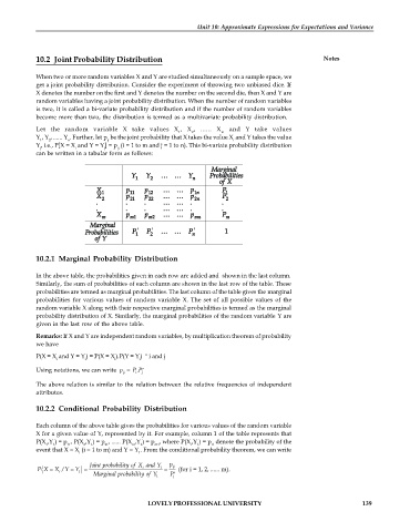
Let the random variable X take values X , X , ...... X and Y take values
1 2 m
Y , Y , ...... Y . Further, let p be the joint probability that X takes the value X and Y takes the value
1 2 n ij i
Y, i.e., P[X = X and Y = Y] = p (i = 1 to m and j = 1 to n). This bi-variate probability distribution
j i j ij
can be written in a tabular form as follows:
Marginal
Y 1 Y 2 ... ... Y n Probabilities
of X
X 1 p 11 p 12 ... ... p 1n P 1
X 2 p 21 p 22 ... ... p 2n P 2
. . . ... ... . .
. . . ... ... . .
X p p ... ... p P
m m1 m2 mn m
Marginal
Probabilities 1  P 2  P ... ... n  P 1
of Y

10.2.1 Marginal Probability Distribution

In the above table, the probabilities given in each row are added and shown in the last column.
Similarly, the sum of probabilities of each column are shown in the last row of the table. These
probabilities are termed as marginal probabilities. The last column of the table gives the marginal
probabilities for various values of random variable X. The set of all possible values of the
random variable X along with their respective marginal probabilities is termed as the marginal
probability distribution of X. Similarly, the marginal probabilities of the random variable Y are
given in the last row of the above table.
Remarks: If X and Y are independent random variables, by multiplication theorem of probability
we have
P(X = X and Y = Y ) = P(X = X).P(Y = Y ) " i and j
i i i i
Using notations, we can write p = i . P P j
ij
The above relation is similar to the relation between the relative frequencies of independent
attributes.

10.2.2 Conditional Probability Distribution

Each column of the above table gives the probabilities for various values of the random variable
X for a given value of Y, represented by it. For example, column 1 of the table represents that
P(X ,Y ) = p , P(X ,Y ) = p , ...... P(X ,Y ) = p , where P(X ,Y ) = p denote the probability of the
1 1 11 2 1 21 m 1 m1 i 1 i1
event that X = X (i = 1 to m) and Y = Y . From the conditional probability theorem, we can write
i 1
Joint probability X and Y p
of
P (X = X /Y = Y ) = i 1 = ij (for i = 1, 2, ...... m).
1
i
Marginal probability Y P
of
1 j
LOVELY PROFESSIONAL UNIVERSITY 139