Page 287 - DMTH404_STATISTICS

Unit 21: Confidence Intervals

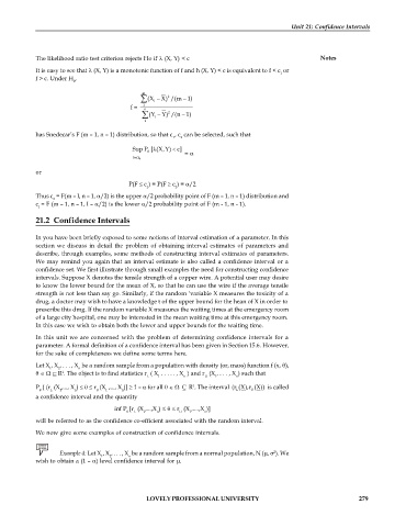
The likelihood ratio test criterion rejects Ho if  (X, Y) < c Notes

It is easy to see that  (X, Y) is a monotonic function of f and h (X, Y) < c is equivalent to f < c or
l
f > c. Under H ,
0
m
2
 (X  X) /(m 1)

i
f = 1 n
2
 (Y  Y) /(n 1)

i
1
has Snedecar’s F (m – 1, n – 1) distribution, so that c , c can be selected, such that
1 2
Sup P [ (X,Y) c]



= 

0
or
P(F  c ) = P(F  c ) = /2
1 2
Thus c = F(m – l, n – 1, /2) is the upper /2 probability point of F (m – 1, n – 1) distribution and
2
c = F (m – 1, n – 1, l – /2) is the lower /2 probability point of F (m - 1, n - 1).
l
21.2 Confidence Intervals
In you have been briefly exposed to some notions of interval estimation of a parameter. In this
section we discuss in detail the problem of obtaining interval estimates of parameters and
describe, through examples, some methods of constructing interval extimates of parameters.
We may remind you again that an interval estimate is also called a confidence interval or a
confidence set. We first illustrate through small examples the need for constructing confidence
intervals. Suppose X denotes the tensile strength of a copper wire. A potential user may desire
to know the lower bound for the mean of X, so that he can use the wire if the average tensile
strength is not less than say go. Similarly, if the random ‘variable X measures the toxicity of a
drug, a doctor may wish to have a knowledge t of the upper bound for the hean of X in order to
prescribe this dmg. If the random variable X measures the waiting times at the emergency room
of a large city hospital, one may be interested in the mean waiting time at this emergency room.
In this case we wish to obtain both the lower and upper bounds for the waiting time.
In this unit we are concerned with the problem of determining confidence intervals for a
parameter. A formal definition of a confidence interval has been given in Section 15.6. However,
for the sake of completeness we define some terms here.
Let X , X , . . . , X be a random sample from a population with density (or, mass) function f (x, ),
1 2 n
   R . The object is to find statistics r ( X . . . . . , X ) and r (X , . . . , X ) such that
1
L 1 n U 1 n
1
P { (r (X ,..., X )    r (X ,..., X )]  1 –  for all    C R . The interval (r (X),r (X)) is called
 L 1 n U 1 n L U
a confidence interval and the quantity
inf P [r (X ,...,X )    r (X ,....,X )]
 L 1 n U 1 n
will be referred to as the confidence co-efficient associated with the random interval.
We now give some examples of construction of confidence intervals.

2
Example 4: Let X , X , . . . , X be a random sample from a normal population, N (,  ). We
1 2 n
wish to obtain a (1 – ) level confidence interval for .

LOVELY PROFESSIONAL UNIVERSITY 279