Page 310 - DMTH404_STATISTICS

Statistics

Notes  6 210 3 60



r    0.99
XY




6 19 9 6 3950 3600
2
1   0.99  


 
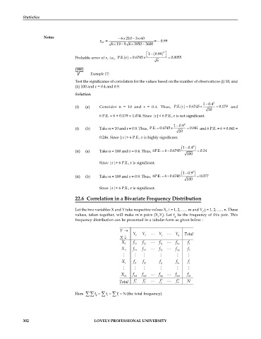
Probable error of r, i.e., P.E. r  0.6745  0.0055
6
Example 12:
Test the significance of correlation for the values based on the number of observations (i) 10, and
(ii) 100 and r = 0.4 and 0.9.
Solution.
1 0.4 2

 
(i) (a) Consider n = 10 and r = 0.4. Thus, P.E. r  0.6745  0.179 and
10
6 P.E. = 6 × 0.179 = 1.074. Since |r|< 6 P.E., r is not significant.
1 0.9 2

(i) (b) Take n = 10 and r = 0.9. Thus, P.E. 0.6745   0.041 and 6 P.E. = 6 × 0.041 =
10
0.246. Since |r|> 6 P.E., r is highly significant.
1 0.4 2 
(ii) (a) Take n = 100 and r = 0.4. Thus, 6P.E. 6 0.6745   0.34
100
Since |r|> 6 P.E., r is significant.

1 0.9 2 
(ii) (b) Take n = 100 and r = 0.9. Thus, 6P.E. 6 0.6745   0.077
100
Since |r|> 6 P.E., r is significant.

22.6 Correlation in a Bivariate Frequency Distribution

Let the two variables X and Y take respective values X , i = 1, 2, ...... m and Y, j = 1, 2, ...... n. These
i j
values, taken together, will make m´n pairs (X ,Y). Let f be the frequency of this pair. This
i j ij
frequency distribution can be presented in a tabular form as given below :
Y 
XB Y 1 Y 2  Y j  Y n Total
X 1 f 11 f 12  f 1j  f 1n f 1
X 2 f 21 f 22  f 2j  f 2n f 2
     
X i f i1 f i2 f ij f in f i
     
X m f m1 f m2  f mj  f mn f m
Total f  1 f  2  f  j  f  n N

ij 
Here  f  f  f  N (the total frequency).
i 
j

302 LOVELY PROFESSIONAL UNIVERSITY